What Is the Peak Hour Effect?

Before 2020, commute demand and resulting traffic congestion were spread more evenly across the week and somewhat more evenly across the morning and afternoon than they are today. There were still clear rush hours, but more people traveled on Mondays and (especially) Fridays, and more riders took trips on either side of the busiest runs.
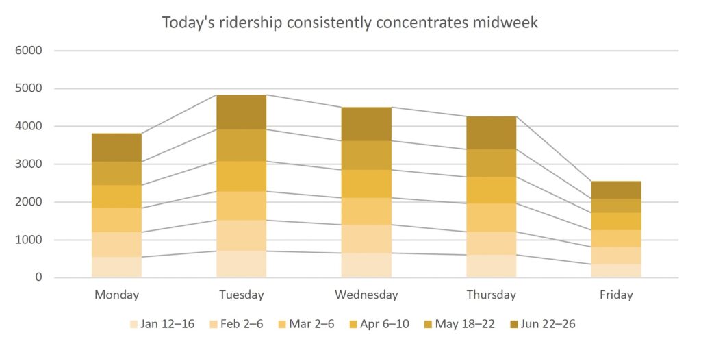
Hybrid work has compressed that demand in two dimensions at once. More commuters now choose the same office days—especially Tuesday and Wednesday—and, on those days, they are also concentrating their trips into a narrower morning and afternoon window. As shown in Figure 1, across six monthly peak-ridership weeks, 68% of all boardings occurred Tuesday through Thursday. Friday accounted for less than 13%. Tuesday had nearly 90% more boardings than Friday across this sample.
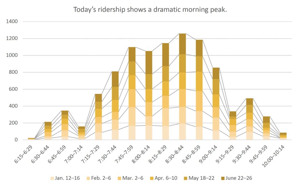
The effect is even more dramatic when we look at time of day rather than day of the week. Across the six sample weeks shown in Figure 2, roughly two out of every three morning boardings occurred during the 90 minutes between 7:45 and 9:15 A.M.
In other words, instead of demand being spread broadly across five days and several hours, an ever larger share of the week’s riders is piling into a handful of trips. That creates what we call the peak hour effect.
So how do we manage this peak hour effect? The ridership charts show when our riders want to travel. The obvious response is to add more departures during these peak periods.
However, every departure added to the schedule requires a physical vehicle and operator to complete the entire trip before they can be used again. You cannot simply move a less-used 7:00 a.m. trip to 8:15 a.m. That same vehicle is already on the road operating at 8:15.

And the problem actually gets worse during peak periods because each vehicle takes longer to come back. A shuttle that can make a relatively quick round trip at 6:30 a.m. may spend substantially longer in traffic at 8:00 a.m. That reduces the number of trips each vehicle can provide precisely when demand is highest.
So there is an unfortunate mismatch: When demand is low, vehicles are relatively easy to reuse. When demand is high, vehicles are harder to reuse.
Adding another trip at the edge of the schedule only require a little additional vehicle operating time. In contrast, adding another trip right in the middle of the peak will require an entirely additional bus and operator, because every existing bus is already occupied. That is why “just move the empty runs to the busy times” cannot solve the problem. The lighter runs are not consuming resources that could be shifted to the peak. The limiting resource during the peak is how many buses and drivers are available to be on the road at once.

Hybrid work therefore makes shuttle service less efficient, even if total ridership has not increased proportionally. In the example above, 100 riders spread across five scheduled trips can be accommodated with a single vehicle. 100 riders all trying to travel at the exact same scheduled time would require four vehicles—even though those three additional vehicles have relatively little to do during the rest of the day.
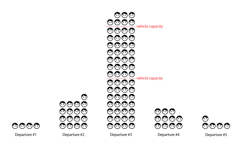
This is actually the same problem a restaurant would have: A restaurant may be able to serve 500 diners over an evening with 50 tables. It cannot serve those same 500 diners all at 7:00 p.m. with those same 50 tables.
Figures 4 and 5 model the same morning ridership. The only thing that has changed in when those 100 riders choose to travel. The more concentrated ridership becomes, the more vehicles we need to carry the same number of people. In other words, peak demand determines our needed fleet size.
Appendix: Table supporting Figure 1
| week | Mon | Tue | Wed | Thu | Fri | total |
|---|---|---|---|---|---|---|
| Jan 12–16, 2026 | 553 | 704 | 655 | 608 | 358 | 2,878 |
| 19% | 24% | 23% | 21% | 12% | ||
| Feb 2–6, 2026 | 653 | 815 | 745 | 607 | 460 | 3,280 |
| 20% | 25% | 23% | 19% | 14% | ||
| Mar 2–6, 2026 | 633 | 762 | 710 | 749 | 442 | 3,296 |
| 19% | 23% | 22% | 23% | 13% | ||
| Apr 6–10, 2026 | 614 | 798 | 743 | 705 | 456 | 3,316 |
| 19% | 24% | 22% | 21% | 14% | ||
| May 18–22, 2026 | 618 | 840 | 770 | 724 | 378 | 3,330 |
| 19% | 25% | 23% | 22% | 11% | ||
| Jun 22–26, 2026 | 750 | 919 | 891 | 876 | 458 | 3,894 |
| 19% | 24% | 23% | 23% | 12% | ||
| All Weeks | 3,821 | 4,838 | 4,514 | 4,269 | 2,552 | 19,994 |
| 19% | 24% | 23% | 21% | 13% |
Appendix: Table supporting Figure 2
time | Jan 12-16 | Feb 2-6 | Mar 2-6 | Apr 6-10 | May 18-22 | Jun 22-26 | total |
|---|---|---|---|---|---|---|---|
| 6:15–6:29 | 0 | 7 | 5 | 3 | 1 | 5 | 21 |
| 6:30–6:44 | 21 | 23 | 49 | 37 | 40 | 42 | 212 |
| 6:45–6:59 | 38 | 73 | 74 | 66 | 46 | 48 | 345 |
| 7:00–7:14 | 17 | 31 | 21 | 23 | 38 | 28 | 158 |
| 7:15–7:29 | 88 | 104 | 78 | 97 | 85 | 91 | 543 |
| 7:30–7:44 | 121 | 119 | 92 | 142 | 155 | 181 | 810 |
| 7:45–7:59 | 165 | 223 | 212 | 167 | 161 | 170 | 1098 |
| 8:00–8:14 | 170 | 109 | 167 | 156 | 176 | 274 | 1052 |
| 8:15–8:29 | 164 | 210 | 148 | 170 | 182 | 272 | 1146 |
| 8:30–8:44 | 191 | 198 | 212 | 197 | 216 | 245 | 1259 |
| 8:45–8:59 | 155 | 185 | 239 | 228 | 183 | 195 | 1185 |
| 9:00–9:14 | 112 | 151 | 122 | 153 | 182 | 136 | 856 |
| 9:15–9:29 | 36 | 62 | 77 | 71 | 30 | 60 | 336 |
| 9:30–9:44 | 94 | 64 | 85 | 78 | 94 | 76 | 491 |
| 9:45–9:59 | 42 | 35 | 39 | 28 | 58 | 76 | 278 |
| 10:00–10:14 | 18 | 8 | 2 | 20 | 14 | 23 | 85 |